kepsilon - 1-D k-epsilon Ocean Turbulence Model

kepsilon is a 1-D tubulence model that integrates mean-flow, and turbulence equations as a function of the vertical. The turbulence model is in base configuration a k-epsilon model. The model includes stratification, waves, breaking waves tke sources, and in the near future bubbles and sediment.

The code is still under development, however it may be of interest to others. The latest version is kepsilon-0.6.0 and is the source code is available as a tarred and gzipped file
kepsilon-0.6.0.tar.gz.
The code is licensed under the GNU GPL This is the first version publicly released.
 

1-D Alongshore Current and Setup Model

This model solves the 1-D alongshore momentum equation which balances wave-forcing against bottom stress and lateral mixing of momentum (e.g.  Longuet-Higgins, 1970; Thornton & Guza, 1986; Church & Thornton, 1993) and is implemented in matlab.  The wave-forcing is given by the wave-transformation model in Church & Thornton (1993).   The wave transformation model is a separate module and can be used independently to calculate wave height distributions.   The modularity also allows different wave models (ie. roller models) to be used.  The lateral mixing is either ignored, or is given by an eddy viscocity formulation where the eddy viscocity is given by Battjes (1975).     There are a number of choices for the parameterization of the bottom stress.  These include the linearized weak-current parameterizations and more complicated nonlinear formulations (Feddersen et al., 1999).

Click on falk-matlabV.tar.gz to download the matlab code.

 

Time-dependent Nearshore Circulation Model

This model is based on the forced and dissipative rigid-lid shallow water equations.   It can be used to study the dynamics of shear waves in the nearshore, and is similar to the model of Allen et al. (1996).    Indeed it has been tested by reproducing features seen in both Allen et al. (1996) and Slinn et al. (1998).  Periodic boundary conditions are used in the alongshore.   Currently, the model is limited to cases where the bathymetry varies only in the cross-shore direction.   A version that works with arbitrary bathymetry is being developed.

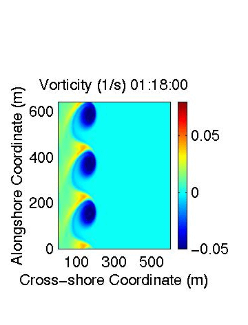
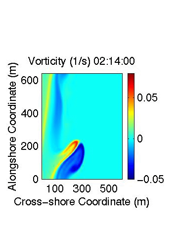
The model can produce vorticity maps (units 1/s), as shown below. The model is run with a planar bathymetry, and an alongshore domain three tiems the most unstable wavelength given from linear stability analysis. The model run was with a small friction coefficient (high Reynolds number), to make the flow is highly unstable. Three aspects of the shear wave evolution are shown below: the initial growth of the instability, the transformation to longer wavelengths, and the offshore ejection of vorticity.
 

Growth and Equilibration This vorticity plot is during the initial growth of the shear waves and corresponds to predictions from linear stability (i.e. Bowen and Holman, 1989). Click here to see an animation (700Kb) of this process. The shear waves become visibile 1:08:00 into the model run. At about 1:20 (after 12 minutes), the shear waves stop growing and begin to equilibrate through the next ten minutes.

Transition to Longer Wavelength Here, the shear waves are undergoing a transition to longer wavelengths. This process is described in Allen et al. (1996). Click here to see an animation (700Kb) of this process. Three equilibrated shear waves appear to undergo a second instability. First, two shear waves merge (starting round 1:50:00) leaving just two shear waves (around 1:55:00) with different magnitudes. The stronger shear waves appears to move faster and catches up with the slower wave around 2:00:00 forming a single wave, or front at the end of the animation.

Ejection of Vorticity After the transition to longer wavelengths, vorticity begins to be intermitently shed from the surf zone offshore. This process is also described by Allen et al. (1996) and Slinn et al. (1998). Shown is the first ejection event which occurs shortly after the transition from three shear waves to a single shear wave. Click here to see an animation (700 Kb) of this process. As the vorticity gets ejected offshore and the water gets deeper, the magnitude of the vorticity increases to conserve potential vorticity. Eventually this eddy dissipates due to bottom friction and also due to biharmonic friction.

A mpeg animation of vorticity evolution which contains the above examples is available. The 20 hour animation (16MB) can downloaded here. A mpeg player such as Image Magik's animate or mpeg_play is required to view the animation.

 For more information on these models and rough documentation contact me at falk@coast.ucsd.edu .
 
 
References

Allen, J. S., P. A. Newberger, and R. A. Holman,  J. Fluid Mech., 310, 181-203, 1996.

Bowen, A. J. and R. A. Holman, J. Geophys. Res., 94, 18,023-18,030, 1989.

Battjes, J. A., Proc of Symp on Modeling Techniques, ASCE, 1050-1061, 1975.

Church, J. C. and E. B. Thornton, Coastal Eng., 20, 1-28, 1993.

Feddersen, F., R. T. Guza, S. Elgar, T. H. C. Herbers, J. Geophys. Res., 105, 8673--8686, 2000.

Longuet-Higgins, M. S., J. Geophys. Res., 75, 6790-6801, 1970.

Slinn, D. N., J. S. Allen, P. A. Newberger, and R. A. Holman, J. Geophys. Res., 103, 18,357-18,379, 1998.

Thornton, E. B. and R. T. Guza, J. Phys. Oceanogr., 16, 1165-1178, 1986.